
To work out the standard deviation, we need to work out the Sxx.
As we have already worked out the Σx, we just need to put that in and square it, then put in the n and times it by the mean we have just worked out squared.
To get the standard deviation, we need to divide the Sxx by n - 1 and then square root it.
s = √389.53 / 11
s = √35.41181818
s = 5.950782989 = 5.95 (2 d.p.)

x̄ + 11.9 = 26.95
x̄ - 11.9 = 3.15
So if the value is below 26.95 or above 3.15, it would be an outlier.
Looking at the table, there is no outliers.

y = 1.8 × 15.05 + 32
y = 59.09
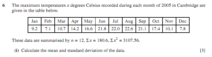
Standard deviation in degrees Celsius = 5.95
y = 1.8 × 5.95 + 32
y = 42.71

The New York temperatures have a greater standard deviation than the Cambridge standard devation.
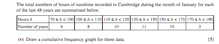
| Upper Bound | 70 | 100 | 110 | 120 | 150 | 170 | 190 |
| Cumulative Frequency | 0 | 6 | 14 | 24 | 35 | 45 | 48 |
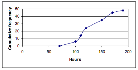
Now all we have to do is put this into graph form. To get full points your graph should look like this...
Remember to...
• Number your graph suitably, e.g. 70 to 190, 0 to 50 (the 0 to 50 scale should not go over 100).
• Label your axis correctly, e.g. "cumulative frequency" and "hours".
• Plot your points correctly e.g. not the mid-point or lower bound.
• Join the dots together either by line or curve. MUST include (70,0).

To do this, we're going to take 90% of the highest cumulative frequency.
Now we're going to look on our graph where 43.2 touches the line. As you can see it's around 160, our estimate of the 90th percentile is 160.
![]()


- Home
- About Us
- Contact
 Online Users
© Copyright 2010-2012 Learn123.co.nr - All rights reserved.